Recurrent Autoencoder v1.0.3

Overview

Recurrent autoencoder for unsupervised feature extraction from multidimensional time-series.

Description

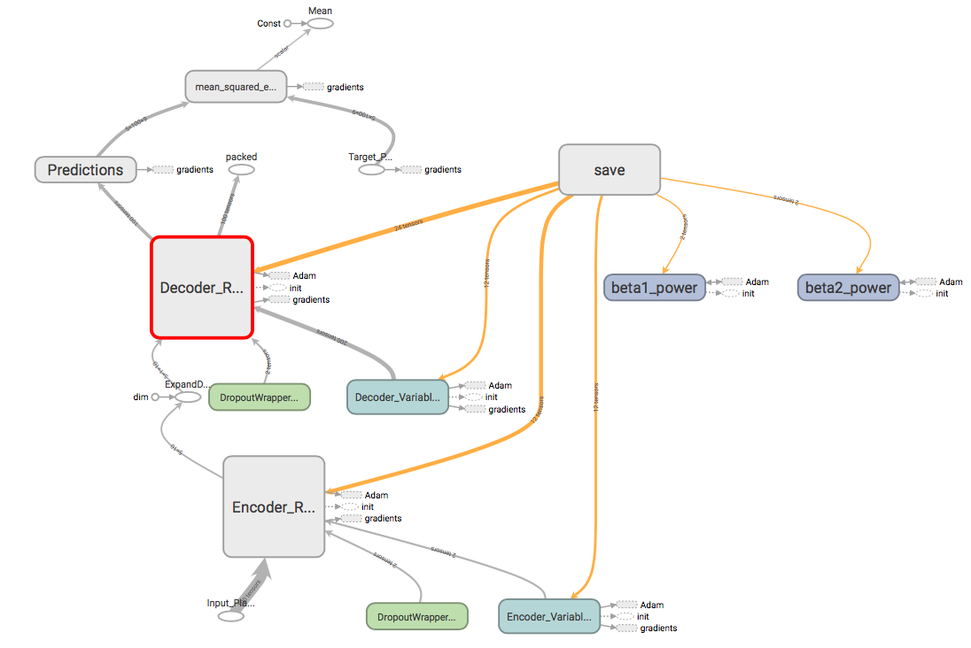
This program implements a recurrent autoencoder for time-series analysis. The input to the program is a .csv file with feature columns. The time-series input is encoded with a single LSTM layer and decoded with a second LSTM layer to recreate the input. The output of the encoder layer feeds in to a single latent layer, which contains a compressed representation of the feature vector. The architecture for the network is the same as illustrated in this paper.

To Run

1. The program is designed to accept .csv files with the following format.

Timestamps	Features	Labels
t = 1	Feature 1 … Feature N	Label 1 … Label M
…	…	…
t = T	Feature 1 … Feature N	Label 1 … Label M

1. Set LSTM parameters/architecture for encoder and decoder in network.py.
2. Set training parameters in autoencoder.py:

   # Training
   NUM_TRAINING = 100		# Number of training batches (balanced minibatches)
   NUM_VALIDATION = 100		# Number of validation batches (balanced minibatches)
   # Learning rate decay
   # Decay type can be 'none', 'exp', 'inv_time', or 'nat_exp'
   DECAY_TYPE = 'exp'		# Set decay type for learning rate
   LEARNING_RATE_INIT = 0.001	# Set initial learning rate for optimizer (default 0.001) (fixed LR for 'none')
   LEARNING_RATE_END = 0.00001	# Set ending learning rate for optimizer
   # Load File
   LOAD_FILE = False 		# Load initial LSTM model from saved checkpoint?
   

3. Set file paths in autoencoder.py:

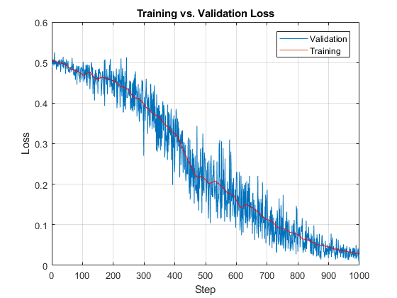
   # Specify filenames
   # Root directory:
   dir_name = "ROOT_DIRECTORY"
   with tf.name_scope("Training_Data"):	# Training dataset
    tDataset = os.path.join(dir_name, "trainingdata.csv")
   with tf.name_scope("Validation_Data"):	# Validation dataset
    vDataset = os.path.join(dir_name, "validationdata.csv")
   with tf.name_scope("Model_Data"):		# Model save/load paths
    load_path = os.path.join(dir_name, "checkpoints/model")		# Load previous model
    save_path = os.path.join(dir_name, "checkpoints/model")		# Save model at each step
    save_path_op = os.path.join(dir_name, "checkpoints/model_op")	# Save optimal model
   with tf.name_scope("Filewriter_Data"):	# Filewriter save path
    filewriter_path = os.path.join(dir_name, "output")
   with tf.name_scope("Output_Data"):		# Output data filenames (.txt)
    # These .txt files will contain loss data for Matlab analysis
    training_loss = os.path.join(dir_name, "training_loss.txt")
    validation_loss = os.path.join(dir_name, "validation_loss.txt")
   

4. Run autoencoder.py. (1) Outputs of the program include training and validation loss .txt files as well as the Tensorboard graph and summaries. The model is saved at each timestep, and the optimal model as per the validation loss is saved separately.
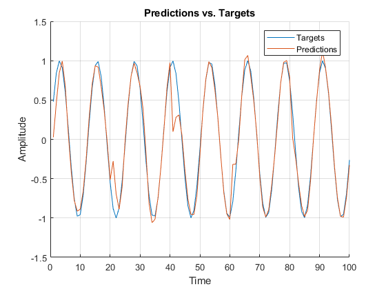
5. (Optional) Run test_bench.py to obtain prediction, target, and latent representation values on a test dataset for the trained model. Ensure that proper filepaths are set before running.

The following is an example of a rapid implementation which encodes the features of a simple sine wave.

Change Log

v1.0.3: Updated to a more generalizable architecture proposed by Cho et. al (2014).

v1.0.2: Updated architecture from that proposed by D. Hsu (2017) to that proposed in this paper, namely one latent layer compressing all time steps and output-feedback into the decoder layer.

Notes

(1) Ensure that you have Tensorflow and Pandas installed. This program was built on Python 3.6 and Tensorflow 1.5.