Probabilistic Graphical Modeling

This collection of MATLAB classes provides an extensible framework for building probabilistic graphical models. Users can define directional or factor graphs, learn or pre-define conditional probability tables, query nodes of the graph, perform variable elimination, and more. The graphs contain the necessary functionality to handle continuous or discrete values, perform message passing, and recursively solve factor graphs.

This framework contains a separate class which builds on the aforementioned functionality to implement hidden Markov modeling (HMM) with hidden state inference using the Viterbi algorithm. A tutorial for implementing HMMs with this framework is provided below.

Table of Contents

1. How to Use
2. Tutorial 1: Directional Graphs
3. Tutorial 2: Factor Graphs
4. Tutorial 3: Hidden Markov Models
5. Additional Help

How to Use

Tutorial 1: Directional Graphs

For this example, we seek to create a hypothetical diagnostic algorithm relating symptoms to an underlying pathology. The possible symptoms are respiratory problems, gastric problems, rash, cough, fatigue, vomiting, and fever; the season (summer or not summer) is included to adjust for seasonality; and the pathologies are flu, food poisoning, hay fever, and pneumonia. We are provided with a data file (joint.dat) which provides the true joint probability distributions over these 12 binary variables, and dataset.dat, which contains samples from the probability distributions in joint.dat.

Graph Creation

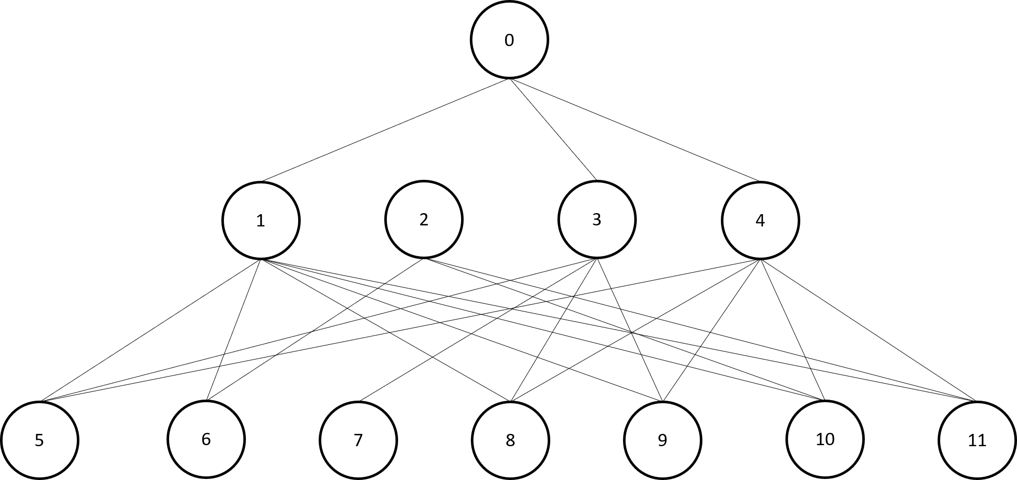
We begin by defining a directional graph of the above variables based on our intuition and domain knowledge. We initialize the nodes of the graph as variable nodes and set dependencies once nodes are all initialized. The nodes and dependencies are then wrapped in a Graph object.

% Initialize graph nodes
summer = Node('isSummer'); hayFever = Node('hasHayFever');
pneumonia = Node('hasPneumonia'); flu = Node('hasFlu');
foodPoisoning = Node('hasFoodPoisoning'); rash = Node('hasRash');
respiratory = Node('hasRespiratoryProblems'); cough = Node('coughs');
gastric = Node('hasGastricProblems'); vomit = Node('vomits');
fatigue = Node('isFatigued'); fever = Node('hasFever');

% Set dependencies
hayFever = hayFever.define('parents', {summer});
pneumonia = pneumonia.define('parents', {summer});
flu = flu.define('parents', {summer});
rash = rash.define('parents', {hayFever});
respiratory = respiratory.define('parents', {hayFever, pneumonia, flu});
cough = cough.define('parents', {hayFever, pneumonia, flu});
gastric = gastric.define('parents', {flu, foodPoisoning});
vomit = vomit.define('parents', {pneumonia, flu, foodPoisoning, gastric});
fatigue = fatigue.define('parents', {hayFever, pneumonia, flu});
fever = fever.define('parents', {pneumonia, flu, foodPoisoning});

% Add nodes to graph
graph = Graph(summer, hayFever, pneumonia, flu, foodPoisoning, rash, respiratory, ...
  cough, gastric, vomit, fatigue, fever);

The resultant graph is shown above. We then build a table from the observations in dataset.dat. The function getObservations() is provided in the tutorials folder.

% Load the dataset
dataset = load('dataset.dat');

% Set variable names to import data table
varnames = {summer.name, flu.name, foodPoisoning.name, hayFever.name, pneumonia.name...
  respiratory.name, gastric.name, rash.name, cough.name, fatigue.name, vomit.name, fever.name};

% Import data table
tab = getObservations(dataset, varnames);

Once the data table is loaded, we use the table to set the conditional probabilities in the graph and return a table of the estimated joint probabilities when we’re done.

% Set conditional probabilities
graph = graph.setConditionals(tab);
% Set assignments
graph = graph.setAssignments();

Querying the Model

By querying our trained model, we can determine the probability that a node will take a value based on certain priors. For instance, we can determine the probability that our patient has the flu given that they have a cough and fever.

query1 = graph.query({flu}, {cough, fever}, {Class.true, Class.true}); disp(query1)

We can also query the value of more than one variable given one or more conditions.

query2 = graph.query({rash, cough, fatigue, vomit, fever}, {pneumonia}, {Class.true}); disp(query2)

Variable Elimination

We may eliminate variables from the graph by providing the node(s) to evaluate, followed by our conditionals, followed by the order in which to perform elimination.

query3 = graph.eliminate({flu}, {cough, fever}, {Class.true, Class.true}, ...
  {cough, fever, respiratory, gastric, rash, fatigue, vomit, foodPoisoning, hayFever, ...
  pneumonia, summer});

Alternatively, we may evaluate more than one node and eliminate the rest.

query4 = graph.eliminate({rash, cough, fatigue, vomit, fever}, {pneumonia}, {Class.true}, ...
  {gastric, respiratory, flu, foodPoisoning, hayFever, pneumonia, summer});

Tutorial 2: Factor Graphs

In this tutorial, we manually create a hidden Markov model (HMM) using factor graphs, a process which has been automated in the next tutorial. We are given a dataset in banana.mat which contains the genetic sequence for a protein found in both humans and bananas. In humans, the genetic sequence is represented by a vector x, where each element x_i is in the set {A, C, G, T}. In bananas, the sequence is represented by the variable y drawn from the same set. The file banana.mat contains the vector x, as well as the emission distributions p(x|h) and p(y|h) along with the transition distribution p(h_t | h_(t-1)). We suppose the initial hidden state is in h = 1 and that there are 5 hidden states such that h is drawn from the set {1, 2, … 5}.

Our task is to use a HMM to infer the most likely banana sequence corresponding to the given human sequence. In the HMM paradigm, this is accomplished by first finding the most likely latent state sequence, and from there inferring the most likely banana sequence. To begin, we load banana.mat and extract the data, converting {A, C, G, T} to {1, 2, 3, 4} for easier analysis.

% Load banana.mat and extract data
load('banana.mat')
xVal = zeros(length(x), 1);
for i = 1:length(x)
    if strcmp(x(i), 'A'); xVal(i) = 1;
    elseif strcmp(x(i), 'C'); xVal(i) = 2;
    elseif strcmp(x(i), 'G'); xVal(i) = 3;
    elseif strcmp(x(i), 'T'); xVal(i) = 4;
    end
end

We initialize the factor nodes and variable nodes as a cell array, with each cell representing a factor node. Since the sequence is 100 base pairs long, we initialize 100 nodes. Though not the most efficient method of HMM implementation (see below), the time-independent property of the HMM will simplify subsequent computation.

% Initialize factor nodes
psi_h = cell(100, 1); psi_x = cell(100, 1); psi_y = cell(100, 1);
h = cell(100, 1); x = cell(100, 1); y = cell(100, 1);

Note that the factor nodes are indicated by psi while the variable nodes lack this prefix. The structure of the HMM graph is illustrated in the image below. Note that the red arrows indicate message passing along the graph.

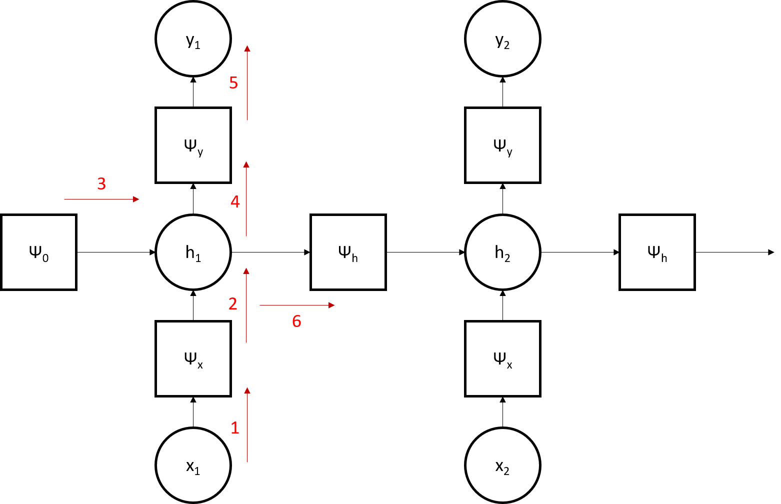We then set the initial conditions of the nodes; factor nodes are initialized with a probability table while variable nodes are not. We start with the initial timestep, then populate the subsequent timesteps.

% Set initial conditions
x{1} = Node('_x1', 'values', {1, 2, 3, 4}); x{1} = x{1}.write(xVal(1));
psi_x{1} = Node('psix_1', 'type', NodeType.factor, 'values', {1, 2, 3, 4, 5}, 'parents', {x{1}});
h{1} = Node('_h1', 'values', {1, 2, 3, 4, 5}, 'parents', {psi_x{1}}); h{1} = h{1}.write(1);
psi_h{1} = Node('psih1', 'type', NodeType.factor, 'values', {1, 2, 3, 4, 5}, 'parents', {h{1}});
psi_y{1} = Node('psiy1', 'type', NodeType.factor, 'values', {1, 2, 3, 4, 5}, 'parents', {h{1}});
y{1} = Node('_y1', 'values', {1, 2, 3, 4}, 'parents', {psi_y{1}});

At this point, we can modify the factor tables with the given probability tables. Since the HMM is time-homogeneous, we create a seed factor using the randomly-generated factor table for each of the three types of factor nodes, then populate the remaining nodes with this seed.

table_xgh = psi_x{1}.factor.table; temp = pxgh'; table_xgh{:, end} = temp(:);
psi_x{1}.factor.table = table_xgh;
table_hgh = psi_h{1}.factor.table; table_hgh{:, end} = phtghtm(:);
psi_h{1}.factor.table = table_hgh;
table_ygh = psi_y{1}.factor.table; table_ygh{:, end} = pygh(:);
psi_y{1}.factor.table = table_ygh;

Next, we populate the remaining nodes in the model.

for i = 2:100
  x{i} = Node(char('_x' + string(i)), 'values', {1, 2, 3, 4}); x{i} = x{i}.write(xVal(i));
  psi_x{i} = Node(char('psix' + string(i)), 'type', NodeType.factor, 'values', {1, 2, 3, 4, 5}, 'parents', {x{i}});
  psi_x{i}.factor.table = table_xgh;
  h{i} = Node(char('_h' + string(i)), 'values', {1, 2, 3, 4, 5}, 'parents', {psi_x{i}, psi_h{i-1}});
  psi_h{i} = Node(char('psih' + string(i)), 'type', NodeType.factor, 'values', {1, 2, 3, 4, 5}, 'parents', {h{i}});
  psi_h{i}.factor.table = table_hgh;
  psi_y{i} = Node(char('psiy' + string(i)), 'type', NodeType.factor, 'values', {1, 2, 3, 4, 5}, 'parents', {h{i}});
  psi_y{i}.factor.table = table_ygh;
  y{i} = Node(char('_y' + string(i)), 'values', {1, 2, 3, 4}, 'parents', {psi_y{i}});
end

Finally, we create and evaluate our factor graph.

graph = Graph([x; psi_x; h; psi_h; psi_y; y]);
graph = graph.solve();

Tutorial 3: Hidden Markov Models (HMM)

In this tutorial, we use a HMM to determine whether each datapoint in a two-dimensional data stream was generated from one of two different Gaussian distributions. In this example, we will define a HMM to generate the data, and run the same model back over the generated data to re-infer the hidden states. To begin, we initialize a blank HMM and set the number of states and observed output variables.

% Set the number of states and observations
markov = markov.set('numStates', 2, 'numObserved', 2);
% Set the names of the hidden states and observations
markov = markov.set('stateNames', {'State1', 'State2'}, 'observedNames', {'Output1', 'Output2'});

Next, we initialized the probability tables. In this case, we start with State 1; we have a 90% chance of remaining in the current state or switching states; and the observations have state-dependent Gaussian distributions: in State 1, Output 1 has mean 1 and Output 2 has mean 2, and vice-versa in State 2.

% Initialize the probability tables
initProb = [1, 0];              % Starting with State 1  
tranProb = [0.9 0.1; 0.1 0.9];  % Propensity to remain in the current state
mu = [1 -1; -1 1];              % The observations have state-dependent Gaussian distributions (mu, sigma)
sigma = zeros(2, 2, 2); sigma(:, :, 1) = 1.0*eye(2); sigma(:, :, 2) = sigma(:, :, 1);
% Set the probability tables in the Markov object
markov = markov.set('initProb', initProb, 'tranProb', tranProb, 'mu', mu, 'sigma', sigma);

We then generate a test sequence of 100 samples and plot the results.

[states, observations] = markov.generate('numSamples', 100, 'plot');

The true hidden states used to generate the data points are captured above. Finally, we use the Viterbi algorithm with the model defined above to re-infer the hidden states from the observations.

viterbi_states = markov.viterbi(observations, 'plot', 'knownStates', states);

In reality of course, the parameters of the HMM must be learned from the data and will not be available a priori. As this model was developed as an extensible framework, such functionality may be added in the future with methods such as the Baum-Welch algorithm. In the meantime, this tutorial serves as an example of the utility of this framework for performing a variety of higher-level tasks with probabilistic graphical models.

Additional Help

Additional help is available for each function in the framework by typing help <Class>.<function> in the command line.