LSTM Network
LSTM network designed for prediction and/or classification. (Tensorflow)
LSTM Network v1.3.5
Overview
LSTM network implemented in Tensorflow designed for time-series prediction and classification. Check out the demo!
Description
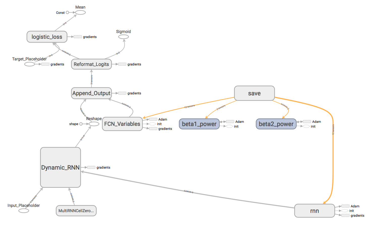
This program is an LSTM network written in Python for Tensorflow. The architecture of the network is fully-customizable within the general framework, namely an LSTM network trained with a truncated BPTT algorithm where the output at each timestep is fed through a fully-connected layer to a variable number of outputs. The the input pipeline can be either rolling-window with offset batches or balanced minibatches and weights updated via truncated BPTT. The error is calculated via tf.nn.softmax_cross_entropy_with_logits_v2 and reduced via tf.train.AdamOptimizer(). This architecture was designed to solve time-series classification of data in two or more categories (one-hot encoded).
Included with the LSTM program are Matlab and Python programs for processing .csv datasets and graphically analyzing the trained network. FeatureExtraction.m contains code designed for pre-processing the input data (including low-pass filtering, RMS, and Fourier analysis), however the data processing section may be adapted for any purpose. NetworkAnalysis.m, contains code designed for visualizing network performance for 3 (one-hot) to 8 (binary-encoded) categories of classification and calculating objective metrics, though it may also be adapted for any purpose.
Features
- Fully-customizable network architecture and training setup.
- Input data processing and trained network validation and analysis code included.
- Ability to save and load checkpoints to pause and continue training.
- Balanced minibatching and rolling-window input pipelines included.
- Advanced hyperparameters such as learning rate decay and dropout layers included.
- Ability to visualize training with Tensorboard and write data to output files for analysis.
- Modular, clean, and commented implementation – highly adaptable for any purpose!
- Plug and Play: It just works.
To Run
- Install Tensorflow.
- Download repository files.
a. In network.py, set the network architecture used in the training and test bench programs.
# Architecture
self.batch_size = 50		# Batch size
self.num_steps = 100		# Max steps for BPTT
self.num_lstm_layers = 2	# Number of LSTM layers
self.num_lstm_hidden = 15	# Number of LSTM hidden units
self.output_classes = 3		# Number of classes / FCL output units
self.input_features = 9		# Number of input features
self.i_keep_prob = 0.9		# Input keep probability / LSTM cell
self.o_keep_prob = 0.9		# Output keep probability / LSTM cell
# Decay type can be 'none', 'exp', 'inv_time', or 'nat_exp'
self.decay_type = 'exp'		# Set decay type for learning rate
self.learning_rate_init = 0.001		# Set initial learning rate for optimizer (default 0.001) (fixed LR for 'none')
self.learning_rate_end = 0.00001	# Set ending learning rate for optimizer
b. In LSTM_Main.py, set training parameters.
# Training
NUM_TRAINING = 1000		# Number of training batches (balanced minibatches)
NUM_VALIDATION = 100		# Number of validation batches (balanced minibatches)
WINDOW_INT_t = 1		# Rolling window step interval for training (rolling window)
WINDOW_INT_v = 1000		# Rolling window step interval for validation (rolling window)
# Load File
LOAD_FILE = False 	# Load initial LSTM model from saved checkpoint?
# Input Pipeline
# Enter "True" for balanced mini-batching and "False" for rolling-window
MINI_BATCH = True
c. Specify files to be used for network training and validation. (1)
# Specify filenames
# Root directory:
dir_name = "/Directory"
with tf.name_scope("Training_Data"):	# Training dataset
 tDataset = os.path.join(dir_name, "data/filename.csv")
with tf.name_scope("Validation_Data"):	# Validation dataset
 vDataset = os.path.join(dir_name, "data/filename")
d. (Optional) Pre-process data with FeatureExtraction.m. Custom pre-processing code may be added in the data processing section. Simply specify number of output classes and whether special analysis should be performed.
LPF = false; % Enable/Disable low-pass filtering
RMS = false; % Enable/Disable RMS calculation
FA = false; % Enable/Disable Fourier Analysis
% Normalize LPF data?
norm_LPF = false;
% Window size for analysis
window_size = 100;
% Fourier analysis results in values for frequency ranges being divided
% into frequency bins and averaged to a discrete value, which is then
% passed as an input feature. Select number of frequency bins:
freq_bins = 9;
% Then select points per fourier bin OR auto-calculate
auto = false;
...
% Specify number of features, classes, and number of timestamp columns
feature_num = 9;
class_num = 3;
timestamp = 1;
...
% Specify output filenames for writing processed data to .csv files:
output_filenames = ["datafile_processed.csv"];
...
% Insert list of filenames from which to import data
filename_list = ["datafile.csv"];
e. Specify file directory for saving network variables, summaries, graph, and training/validation loss.
with tf.name_scope("Model_Data"): # Model save path load_path = os.path.join(dir_name, "checkpoints/model") # Load previous model save_path = os.path.join(dir_name, "checkpoints/model") # Save model at each step save_path_op = os.path.join(dir_name, "checkpoints/model_op") # Save optimal model with tf.name_scope("Filewriter_Data"): # Filewriter save path filewriter_path = os.path.join(dir_name, "output") with tf.name_scope("Output_Data"): # Output data filenames (.txt) # These .txt files will contain loss data for Matlab analysis training_loss = os.path.join(dir_name, "training_loss.txt") validation_loss = os.path.join(dir_name, "validation_loss.txt") - Using the terminal or command window, run the python script LSTM_main.py. (2) (3) (4)
- (Optional) Analyze network parameters using Tensorboard.
- (Optional) Run test_bench.py to analyze trained network outputs for a validation dataset (predictions and targets saved as .txt files). Ensure to select the correct filepaths as shown below. The network architecture is automatically drawn from network.py and weights are automatically adjusted if drop layers were used.
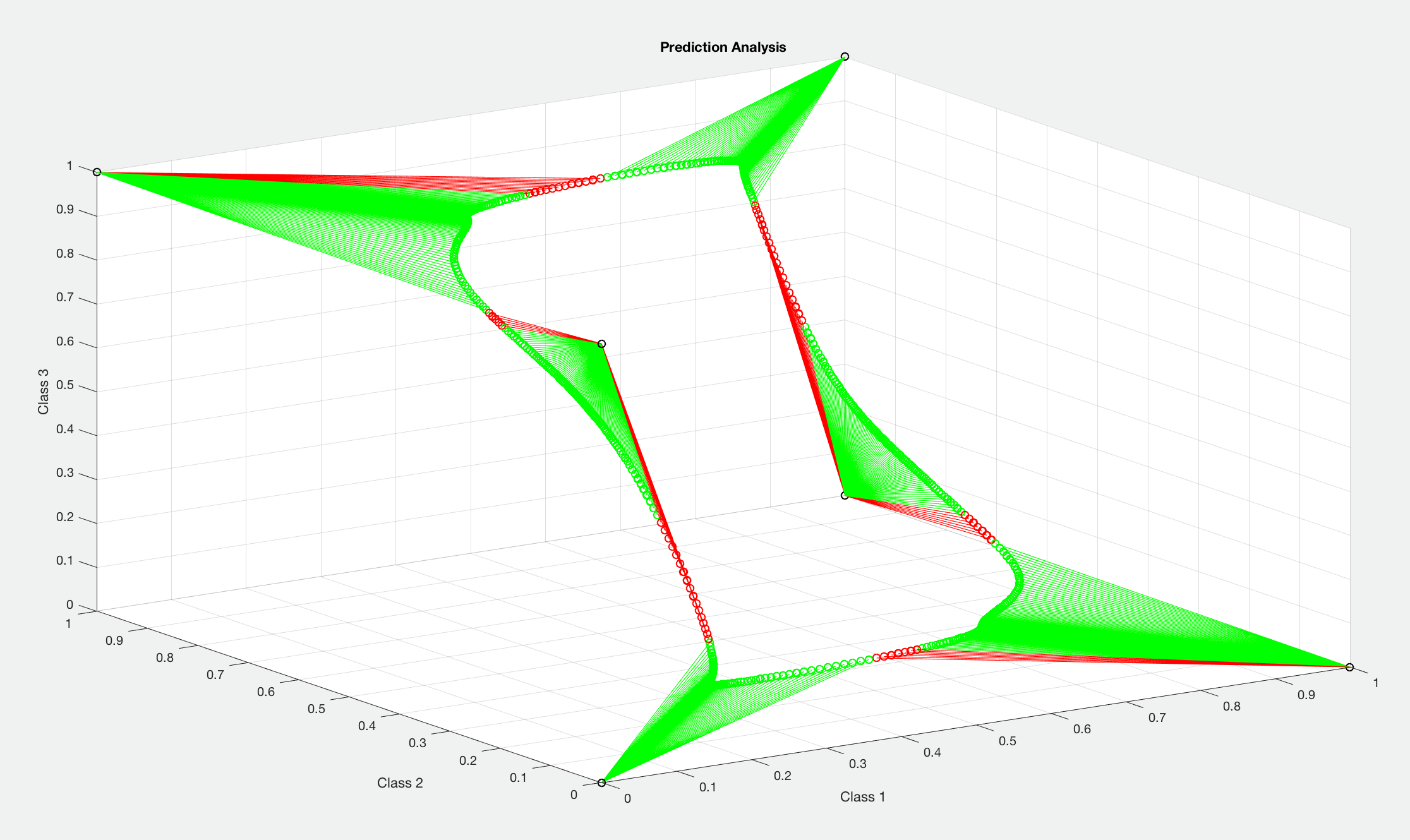
dir_name = "/Users/username" with tf.name_scope("Training_Data"): # Testing dataset Dataset = os.path.join(dir_name, "datafile.csv") with tf.name_scope("Model_Data"): # Model load path load_path = os.path.join(dir_name, "checkpoints/model") with tf.name_scope("Filewriter_Data"): # Filewriter save path filewriter_path = os.path.join(dir_name, "output") with tf.name_scope("Output_Data"): # Output data filenames (.txt) # These .txt files will contain prediction and target data respectively for Matlab analysis prediction_file = os.path.join(dir_name, "predictions.txt") target_file = os.path.join(dir_name, "targets.txt") - (Optional) Run NetworkAnalysis.m to graphically analyze predictions and targets for the trained network and/or add custom code in the data analysis section. The code provided obtains one-hot vectors from predictions as well as integer classifications for subsequent data analysis and visualization. The program outputs sensitivity, specificity, precision, recall, and F1 for each class as well as the ROC curve and AUROC for a specified class. Simply specify preferences in the header.
% Specify number of classes
numClasses = 3;
% Toggle data visualization
visualize = true;
% Toggle ROC curve generation
ROC = true;
% Select class for which to generate ROC curve
rocClass = 2;
Update Log
v1.3.5: Added support for several types of learning rate decay. Minibatch training and validation losses are written to output files for improved analysis of network performance. Improved network analysis and feature extraction scripts. Updated NetworkAnalysis.m metrics reporting and added ROC analysis.
v1.3.1 - v1.3.4: Improved user interface and ability to handle a variable number of output classes as one-hot vectors. Introduced balanced minibatch input pipeline. Added ability to save optimal model state as checkpoint. Included network.py so that network architecture is preserved across all python files. Bug fixes and improvements.
v1.2.1 - v1.2.4: Improved exception handling and added ability to load partially-trained networks to resume training. Added ability to conditionally call optimizer when running the session to mitigate class imbalance. Added capability for >2 target categories (vs. binary classification) and rolling window step interval for decreasing training time overfitting likelihood. Updated test bench to output predictions and targets to .txt file for Matlab analysis. Added Matlab program for analysis of the trained LSTM network.
v1.1.1 - v1.2.0: Updated mean-squared error loss approach to sigmoid cross-entropy. Added test bench program for running trained network on a validation dataset. Added feature extraction Matlab script for data pre-processing. Added ability to save network states and LSTM cell dropout wrappers. Added rolling-window input pipeline.
Notes
(1) To use the stock input pipeline, the training datafiles must be CSV files with columns in the following arrangement:
| TIMESTAMP | FEATURE_1 … FEATURE_N | LABEL_1 … LABEL_M |
|---|---|---|
| … | … | … |
Note that the timestamp column is ignored by default and any column heading should be removed, as these may be read as input data. The number of feature and label columns may be variable and is set by the user-defined parameters self.input_features and self.output_classes respectively in network.py. The labels should be a one-hot vector when using the provided softmax classifier.
(2) The program will output training loss, validation loss, percent completion and predictions/targets at each mini-batch. It will also output the current learning rate and time remaining at the specified number of steps. To adjust these display settings, edit the lines below:
[345] # Conditional statement for validation and printing
[346] if step % 50 == 0:
...
[397] # Conditional statement for calculating time remaining and percent completion
[398] if step % 10 == 0:
(3) As of v1.1.1, ensure you have installed pandas!
(4) As of v1.2.3, ensure that you have the most recent version of Tensorflow installed (1.5).
References
(1) Tensorflow’s Recurrent Neural Network Tutorials